Figure 1. EPS Component Models and EPS System Representation
97543
POWER SIZING AND POWER PERFORMANCE SIMULATION TOOLS
FOR GENERAL EPS ANALYSES
Patrick G. Bailey
Lockheed Martin Missiles and Space Company
P.O Box 3504
Sunnyvale, CA 94088-3504
408-743-0301, Patrick.Bailey@lmco.com
Jack Lovgren
Lockheed Martin Missiles and Space Company
P.O Box 3504
Sunnyvale, CA 94088-3504
408-743-7222, Jack.Lovgren@lmco.com
Presented at the
32nd Intersociety Energy Conversion Engineering Conference
INTERNATIONAL ENERGY TECHNOLOGY
July 27 - August 1, 1997
Honolulu, Hawaii
Invited Paper
[The figures herein were scanned in from the IECEC-97 Proceedings, AIChE, Volume 1, pages 262-267]
97543
POWER SIZING AND POWER PERFORMANCE SIMULATION TOOLS
FOR GENERAL EPS ANALYSES
Patrick G. Bailey
Lockheed Martin Missiles & Space
P.O Box 3504
Sunnyvale, CA 94088-3504
408-743-0301, Patrick.Bailey@lmco.com
Jack Lovgren
Lockheed Martin Missiles & Space
P.O Box 3504
Sunnyvale, CA 94088-3504
408-743-7222, Jack.Lovgren@lmco.com
ABSTRACT
Several Electric Power System modeling and simulation tools have been developed at Lockheed Martin that are being used in detailed EPS component designs and also in detailed EPS transient performance analyses. A consistent set of very detailed EPS components are used within each of the tools. The components can be chosen by the user to be very simple, such as time-averaged component values, or extremely detailed, such as instantaneous non-linear models that have been verified against component test data. These tools have been used for a variety of satellite mission studies, and have been successfully used in both EPS component sizing studies and in detailed component and system transient performance calculations. Several EPS systems models are presented for discussion, the EPS component models are summarized in detail, and example results are included.
INTRODUCTION AND BACKGROUND
Electric Power System (EPS) modeling and simulation tools continue to play a very significant role in the design and sizing of Electronic Power System components for both general satellite applications and various ground-based electric power generation stations. Most sizing and simulation tools utilize simplistic models and time-averaged power requirements to arrive at best-guess component sizes and capabilities, which are then over-sized by selected design engineering margins depending upon their specific application.
Lockheed Martin has developed detailed simulation models for each component and each subcomponent of the entire general EPS to allow detailed non-linear simulations, design analyses, component sizing, and transient performance for all EPS applications of interest. As these models are modular and interconnect, other more simplistic models may also be used to verify the results from other analyses. These tools are being used to size and study several planned missions A summary of the capabilities of the component models and detailed example results are given in this paper. EPS components including the battery cells and solar array cells can be evaluated and sized for any life, eclipse, and load combination. Using more historic and simpler models for the EPS components, these detailed results can be easily compared to design studies performed several years ago. It is found that the use of these detailed models can result in EPS designs that are of significant lower cost and lighter weight than those designed by other design tools.
EPS SIMULATIONS
A detailed EPS simulation model should provide the following results:
ï Ability to Calculate at Any Orbital Position
ï Ability to Calculate at Any Sun Angle or Sun Intensity
ï Balanced and Converged EPS Architecture Loads
ï Instantaneous Voltages and Currents
ï Instantaneous Temperature
ï Instantaneous Heat Transfer
ï Instantaneous Thermal Effects
ï Transient Behavior
ï Component Aging
ï Launch Effects
ï Orbital Cycle Effects
ï Life Cycle Effects
EPS Simulation Tools are generally divided into two classes:
ï EPS Component Sizing Tools
ï EPS System Transient Performance Tools.
The EPS Component Sizing Tools allow the input of average orbital component parameters to determine average component sizes and weights. The inputs may include: EPS life, sun and eclipse profile, component average temperatures, cable lengths and sizes, and battery size and composition. The outputs may include: component sizes, dimensions, weights, costs, electronic cards types and counts, solar array series and parallel cell counts, battery sizing, and power use summaries.
Depending upon what input parameters are specified, the user should be able to specify what output variables are to be calculated. This allows the input and output parameters to be chosen by the user.
The EPS System Transient Performance Tools. allow the input of instantaneous orbital, sunlight, and load conditions to determine the instantaneous operating characteristics in each of the EPS components, such as voltage, current, temperature, and heat transfer. Performing these calculations for each position over the orbit or several orbits in a mission will result in the time-dependent, transient EPS response of each component within the EPS. The inputs may include: EPS life, sun angle and intensity, load, component detailed designs, component temperatures, and battery charging methods. The outputs may include: voltages and currents anywhere in the EPS, battery depth-of-discharge, maximum depth-of-discharge, battery heat generation, and EPS temperatures.
EPS COMPONENT MODELS
The component models should also contain the necessary data to be able to provide cost, size, weight, performance, reliability, technology, and power consumption information. These data can be included to make each component scalable for any defined application.
In the past, several EPS modeling tools have been written in FORTRAN or C code, allowing the defined outputs to be easily calculated from the defined inputs. In these codes, the solution is then determined by defined sequential causality; i.e. in the manner in which the equations are written. A drawback of the use of these models is that the input and output variables are rigidly defined and linked by that causality. If the user wishes to arbitrarily choose what the input and output parameters are for a given component model, then those EPS codes must include the proper decision trees to select which causality model (e.g. which subroutine) is to be used, and provide such a model for each case that may be encountered. When updating the equations of such a model, all the equations in each causality model must also be carefully updated. This is not difficult to do for most linear subsystem models. However, it is extremely difficult to do for non-linear subsystem or component models.
With the advent of the high speed desk top computer, other EPS models are now being written in SPICE, PSPICE, and in EXCEL (and similar equivalent modeling platforms). These application platforms allow the component models to be each identified and linked by defined equations, that are then iteratively solved until a converged solution is found. The use of these platforms allows greater flexibility and complexity in the way in which the components are modeled, and also allow the inclusion of non-linear and feedback effects which cannot be easily incorporated into the above FORTRAN or C program simulations. However, the numerical convergence to a steady-state or equilibrium solution at each time-step may require a much longer period of time than that of the direct sequential methods above, and in some cases, depending upon the application platform and the models, the solution may not even converge!
NUMERICAL SOLUTION CONCERNS
Several comparison studies have been performed using the PSPICE platform and the EXCEL spreadsheet application to simulate the complex, non-linear EPS component models used as described below. It was found that while the PSPICE application was very useful in several respects and did solve the non-linear convergence and numeric solution problems, it can also generate very large and lengthy output files that are very difficult to process, edit, and understand. On the other hand, the use of the automatic conversion algorithm inherent within the EXCEL application program is also able to easily converge and solve these complex systems without the generation of such overhead. In addition, the use of Visual Basic within EXCEL 5.0 has made the use of this application much easier (over the use of the old EXCEL macros) and much faster. While the use of such applications does guarantee a convergence to a system solution, experience has shown that a proper numerical convergence is almost always reached. Also, the first converged solution may not be the best solution from an engineering and design standpoint. Several trade studies are usually performed to insure that the chosen EPS component types, sizes, and operational characteristics are all adequate for all of the mission and operational requirements, before detailed steady-state and transient performance studies are performed.
The use of EXCEL 5.0 also allows the automatic presentation of plots of the results which has been found to be an invaluable asset to the design engineer and the EPS power systems analyst.
EPS ARCHITECTURE TYPES
The EPS architecture types that have been incorporated into the EPS tools include:
ï Battery dominated bus with direct connect, series switched solar array
segments
ï Battery dominated bus with peak power tracked solar array
ï Sunlit regulated bus with direct connect, series switched solar array
segments
ï Sunlit regulated bus with peak power tracked solar array
ï Fully regulated bus with direct connect, parallel shunted solar
array segments, and battery charge / discharge regulators
connected to the regulated bus
These architectures have been used to model some of the LMMS EPS systems, such as: LM700, MILSTAR, several Peak Power Tracker based systems, A-2100, and A-2100M.
EPS COMPONENTS AND MODELS
EPS System Components
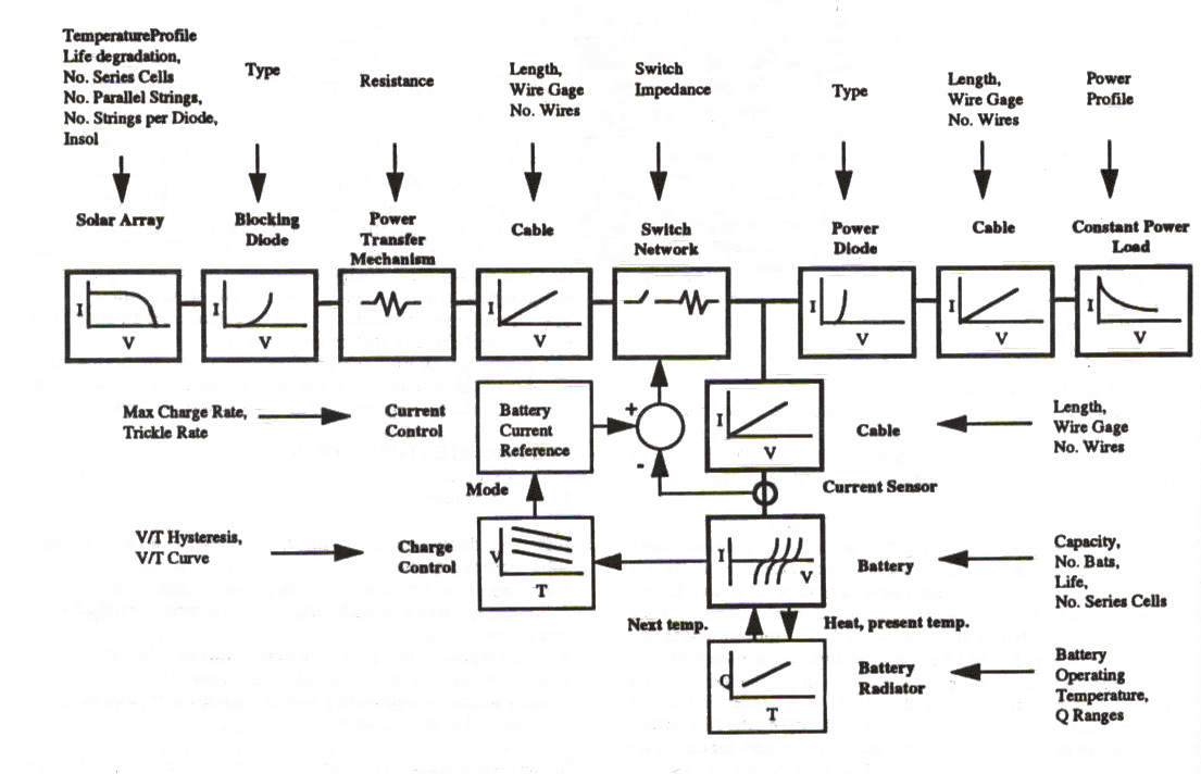
A summary representation of the general EPS that can be defined by the EPS component models used is shown in Figure 1.
Each of the EPS components shown in Figure 1 are now summarized, including a listing of all of the input and output parameters which define that particular component. Mission and orbital characteristics are included to provide the sunlight and eclipse driving functions to particular component models.
Mission Characteristics
The Mission Characteristics input into the Model are:
Average Life (yrs)
Average Sun Load (W)
Average Eclipse Load (W)
Transient Sunlight Intensity (%)
Transient Sunlight Angle (Deg.)
Transient Load Required
Transient Radiator Load Allowed
Figure 1. EPS Component Models and EPS System Representation
Orbit Characteristics
The Orbit Characteristics input into the Model are:
Duration (Min)
Eclipse (Min)
GEO (Y or N)
Equinox:
Intensity of Sun
Normal Inclination (Deg.)
Inclination Error (Deg.)
Solstice:
Intensity of Sun
Normal Inclination (Deg.)
Inclination Error (Deg.)
Dual Axis Tracking (Y or N)
Charge or Discharge in Sun (Y or N)
Charge Load (W)
Discharge Load (W)
Solar Array
Each solar array is defined as a group of strings (connected in parallel) of a number of solar array cells (connected in series). Each array is considered to be built from one type of solar array cell. Currently, two separate arrays can be defined and utilized within the EPS. Each solar array cell is modeled upon the well known Hughes Solar Cell Model that relates the cell voltage to the current for a given temperature and solar illumination. This relationship is illustrated in Figure 1.
The solar array model is entered, pre-aged, into a table of available solar cell types available for simulation. The degradation analysis for solar cells, being unique to each specific application, is performed using a specialized solar cell degradation model. The system model accepts the user-selected modeling parameters from the solar cell library and provides run time adjustment of temperature and operating point of the selected cell configuration. An example of a solar cell string configuration over a range of temperatures (the higher voltage curves are colder) and operating voltages is given in Figure 2.
The inputs to the EPS Solar Array Component Model are:
Fraction of SA Provided by SA 1
Fraction of SA Provided by SA 2
Maximum Number of Solar Array Groups
Number of Space SA Circuit Groups
For each SA:
Solar Cell Type
Number of Cells per String
Number of Strings per Group
Operating Temperature (C)
Testing temperature (C)
Blocking Diode
The blocking diodes are represented by the ? relationship relating the diode's voltage to current flow. This relationship is illustrated in Figure 1.
Resistance
The power loss within each component is given in terms of its electrical resistance, as illustrated in Figure 1.
Solar Array Switching Network
An automatic solar array switching network (SASN) is also modeled that can be used to automatically switch groups or strings of cells off and on as determined by the power demands of the EPS system. This is illustrated in Figure 1.
Power Junction Box
PRU or PSDU
Determined by the EPS Architecture Selection
Battery
Number of Batteries
Sequenced Charging (Y or N)
Type of Battery Cells
Number of Battery Cells
Number of Failed Cells
Required Capacity (AHr)
Voltage
Maximum Depth-of-Discharge (%)
Available Charge Time (Min)
Available Discharge Time (Min)
Operating Temperature (C)
Recharge Ratio
The battery component model allows the use of a 2-D characteristic surface to model the battery voltage as a function of both the depth-of-discharge and the discharge-rate at a specific temperature. The battery model accepts both life aging parameters and run-time parameters. Life adjustments are made for calendar life, cycle life, average life temperature and average life depth of discharge. Run time parameters include instantaneous current, instantaneous temperature, and instantaneous depth of discharge. Outputs include instantaneous voltage and instantaneous charge efficiency, and are adjusted according to certain low frequency time dependent behaviors of batteries. Figure 3 illustrates an example battery voltage as a function of rate and depth of discharge, with temperature held constant, life degradation set to beginning of life, and low frequency time dynamic effects assumed to be timed out (e.g. DC rather than dynamic conditions).
Current Control
Simulation according to the control laws present in the selected architecture.
Charge Control
Ampere hour integration, pressure, and VT are supported, along with an "ideal" charge control algorithm.
Battery Radiator
A generic battery cooling algorithm is employed, although the exact field of
view, and therefore the precise cooling profile, is not known.
Cabling
For Each Cabling Connection:
Length (ft)
Gauge (AWG)
Number of parallel Conductors
Cable temperature
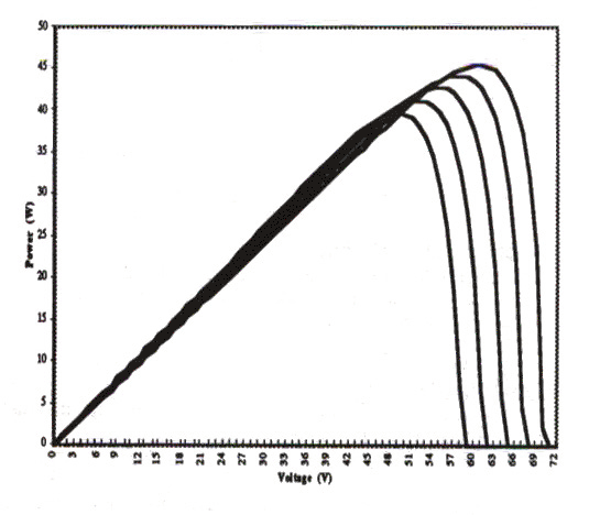
Figure 2. Solar Array Power vs. Voltage for Various Temperatures
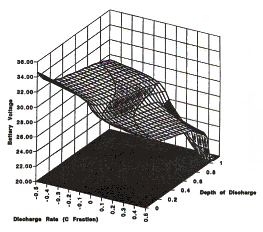
Figure 3. Battery Voltage Model (Generic) for one Temperature
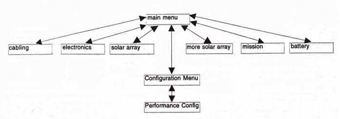
Figure 4. EPS Tools Operational Capabilities
Electronic Data Module
Number of Various Electronic Cards to be Used
Number of Various Electronic Controllers to be Used
Battery reconditioning (Y or N)
Etc.
Power Diode
The power diode relates the current flowing through the diode to the voltage across the diode as shown in Figure 1.
Load
The EPS load is defined by orbital averaged sun and eclipsed loads and by a time-dependent load profile for each desired position in orbit. This component is illustrated in Figure 1.
EXAMPLE MODELS AND DATA
The operational capabilities of the EPS Tools are illustrated above in Figure 4.
EXAMPLE RESULTS
The use of these tools has also produced some rather surprising results, such as:
1. A certain load/sunlight pattern was found to cause battery discharge in
sunlight, resulting in a declining battery state-of-charge;
2. A deployment delay was found advantageous in a certain scenario due to the
timing of load profile and mission eclipse patterns; and
3. A PSDU architecture was found more advantageous than a Power Tracker design
for the same mission due to the interactions of the high peak-to-average power
profile and the battery discharge profile that occurred during the non-eclipse
portion of the mission.
An arbitrary EPS system is analyzed, and transient performance analysis results are shown in Figures 5 through 9.
A battery dominated bus architecture with a sun-tracking solar array is modeled with no solar array switching for two orbital cycles of 100 minutes each. Each cycle consists of 35 minutes eclipse followed by 65 minutes of sunlight. The percent amount of light impacting perpendicular to the solar array (Insol), and the resulting solar array temperature for these two orbits is shown in Figure 5. It is noted that the solar array temperature varies greatly, from about -75 C to about +75 C during these cycles.
The load power required for the Bus, Communications, and Payload as chosen for this study are shown in Figure 6. The upper curve represents the total power required from the EPS. This power profile was chosen to demonstrate the effect of having two payload power pulses during the first orbit (one beginning in eclipse), and a large 3X over-power pulse (triangular) during the second cycle. The resulting battery current required to compensate for the total load and the battery charging efficiency are shown in Figure 7. It is seen that in both cycles, the battery supports the load during the eclipse, and recharges in the sunlight, and follows the shape of the required load power.
The resulting battery voltage and the battery depth-of-discharge (from 0%) are both shown in Figure 8. It is seen that the battery discharges and recharges based on the summation (integral) of the load power times insol, and that the battery fully recharges before the end of each cycle (As supported by a zero battery current after the battery is fully recharged, as seen in Figure 7.). It is also seen that the battery voltage varies quite strongly during this transient, as much as nearly ten volts during these two cycles. It is recalled that the battery voltage is part of the non-linear response of the battery that is solved for and converged during each time step during this analysis. The resulting battery temperature and heat created are shown in Figure 9. Although the temperature of the battery is shown to vary only a few degrees, the heat that the battery generates is as much as 220 Watts during the first eclipse cycle.
These arbitrary results are provided to show the capabilities of the EPS tools in calculating detailed and consistent EPS sizing and transient studies. The results shown are not intended to represent any real or proposed EPS system or satellite mission.
SUMMARY AND CONCLUSIONS
Several EPS simulation models are in use today for both individual EPS component sizing, and EPS system transient performance. Simple models can be coded in digital programs, and generally give lumped-parameter or conservative results that are usually increased by engineering margins. Detailed non-linear EPS models can be made that model and reproduce actual test data; however, the use of these models in digital simulations can be very difficult, and the results can be very suspect.
An EPS Sizing Tool and an EPS Transient Performance Tool have been developed at Lockheed martin for use in general orbital satellite and ground-based power station applications. The tools allow the use of complex, non-linear EPS component models whose results reproduce actual test data. EPS simulations are constructed from these models for both component sizing and performance studies. The use of EXCEL allows general user selected input and output variables while maintaining modularity and numerical convergence. The use of Visual Basic allows a marked increase in real-time simulation speed and in automatic detailed graphical results. The EPS component models are shown to reproduce actual test data, and the EPS system models using the same components are shown to produce accurate results in both EPS component sizing and transient analysis calculations. Results from other studies have shown the models to reproduce other contractor's data and results almost exactly.
The EPS Tools are being used in a variety of EPS component sizing and performance calculations for various Programs, Architectures, and Missions within Lockheed Martin.
ACKNOWLEDGMENTS
The support and cooperation of the Lockheed Martin Missiles and Space Products Center is gratefully acknowledged.
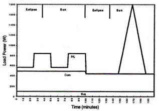
Figure 5. Representative EPS Transient Results: Two Cycle Load Power Profile
(W) (Chosen) vs. mission time (m).
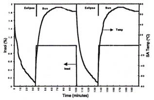
Figure 6. Representative EPS Transient Results. Solar Array Insol and
Temperature (C) vs. mission time (m).
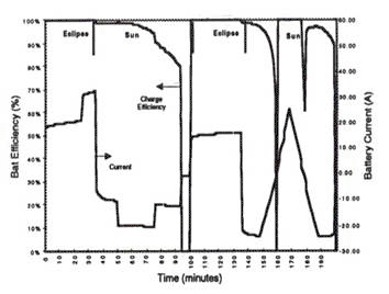
Figure 7. Representative EPS Transient Results. Battery Charge Efficiency (%)
and Current (A) vs. mission time (m).
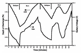
Figure 8. Representative EPS Transient Results. Battery DOD (%) and Voltage
(V) vs. mission time (m).
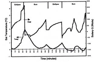
Figure 9. Representative EPS Transient Results. Battery Temperature (C) and
Battery Heat (W) vs. mission time (m).
www.padrak.com/pgb/IECEC_1997_EPS.html
February 12, 2004.